Bayesian Inference
ititer uses Bayesian inference to infer posterior distributions of sigmoid curve parameters.
Formally, the response of sample i, \(y_i\), is modelled as a function of log dilution using a four parameter logistic curve, \(x_i\):
Parameters are interpreted as follows:
\(a\) - horizontal location of the sigmoid
\(b\) - gradient at the inflection point
\(c\) - minimum response
\(d\) - difference between minimum and maximum
Parameters can either be set a priori, inferred using full pooling (yielding a single distribution from all samples), or inferred using partial pooling (where each sample gets its own posterior distribution).
Standardizing
Log dilution is standardized to have mean of zero and standard deviation of one for inference.
Response is standardized to have a minimum of 0 and maximum of 1.
Priors
Weakly informative priors are used by default throughout. When parameters a, b, and c are fully pooled, they given a prior of \(\text{dnorm}(0, 1)\). When a, b, and c are partially pooled across samples, s, they are given priors of:
To prevent redundancy between the values of c and d, d is constrained to be positive. When it is fully pooled: \(d \sim \text{dexp}(1)\). When it is partially pooled:
These priors will be applicable for most users.
Partial pooling for a, full pooling for b and d, and setting c=0 gives the following prior predictive distribution:
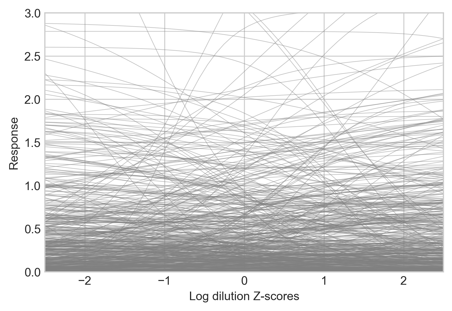
Code used to generate this figure:
import numpy as np
import matplotlib.pyplot as plt
import ititer as it


df = it.load_example_data()
df["Log Dilution"] = it.titer_to_index(df["Dilution"], start=40, fold=4)

sigmoid = it.Sigmoid().fit(
    data=df,
    response="OD",
    sample_labels="Sample",
    log_dilution="Log Dilution",
    prior_predictive=True,
)

x = np.linspace(-2.5, 2.5).reshape(-1, 1)
y = it.inverse_logit(
    x=x,
    a=sigmoid.prior_predictive["a"][:, 0],
    b=sigmoid.prior_predictive["b"],
    c=0,
    d=sigmoid.prior_predictive["d"],
)

plt.plot(x, y, c="grey", alpha=0.5, lw=0.5)
plt.xlabel("Log dilution Z-scores")
plt.ylabel("Response")
plt.ylim(0, 3)
plt.xlim(-2.5, 2.5)
plt.savefig("prior-predictive.png", bbox_inches="tight", dpi=300)