Tutorial
Load some example data using ititer and look at the first 10 rows:
import ititer as it
df = it.load_example_data()
df.head(10)
Sample |
OD |
Dilution |
|---|---|---|
21-P0004-v001sr01 |
1.371 |
40 |
21-P0004-v001sr01 |
0.981 |
160 |
21-P0004-v001sr01 |
0.535 |
640 |
21-P0004-v001sr01 |
0.182 |
2560 |
21-P0004-v001sr01 |
0.064 |
10240 |
21-P0004-v001sr01 |
0.027 |
40960 |
21-P0004-v001sr01 |
0.015 |
163840 |
21-P0004-v001sr01 |
0.010 |
655360 |
21-P0034-v001sr01 |
0.948 |
40 |
21-P0034-v001sr01 |
0.452 |
160 |
Each row contains information about a single OD measurement; the sample, OD value and the dilution factor.
The measurements for the first sample, 21-P0004-v001sr01 are in the first 8 rows, followed by those for 21-P0034-v001sr01.
This is known as long format data.
Wide format data
If your data is in wide format,
for instance perhaps each row contains OD values at different dilutions for a single sample ,
then use pandas.DataFrame.melt() to generate a long format DataFrame.
Example wide format data:
Sample |
40 |
160 |
640 |
2560 |
10240 |
40960 |
163840 |
655360 |
|---|---|---|---|---|---|---|---|---|
21-P0004-v001sr01 |
1.371 |
0.981 |
0.535 |
0.182 |
0.064 |
0.027 |
0.015 |
0.01 |
21-P0034-v001sr01 |
0.948 |
0.452 |
0.185 |
0.043 |
0.016 |
0.004 |
0.002 |
-0.001 |
21-P0050-v001sr01 |
1.418 |
1.253 |
0.972 |
0.393 |
0.152 |
0.049 |
0.018 |
0.011 |
For a DataFrame exactly like this the call to melt would be:
df.reset_index().melt(id_vars="Sample", var_name="Dilution", value_name="OD")
Log transform dilutions
Next, we need to transform the dilutions (which increase logarithmically) to values that increase linearly. This will mean that when the data are plotted, the values will be evenly spaced on the x-axis.
There is a helper function for doing this called titer_to_index().
The titer argument is the dilutions, start is the first dilution in the dilution series, and fold sets the fold change in concentration at each step in the dilution series.
We can call the function and store the returned value as a new column in our DataFrame:
df["Log Dilution"] = it.titer_to_index(titer=df["Dilution"], start=40, fold=4)
Fit curves
We are now ready to fit sigmoid curves for each sample.
We want partial pooling between samples for inference of the a parameter to give us one estimate of a for each sample.
We know a priori that the response will be 0 at a theoretical infinite dilution, so we can set c=0.
We will use full pooling for b and d because we expect the gradient of the sigmoid curve (b) and its height above baseline (d) to be the same across samples.
We make a new Sigmoid object that has these properties:
sigmoid = it.Sigmoid(a="partial", b="full", c=0, d="full")
Now we call the fit() method to infer the posterior distributions of the model parameters, and supply the data from our long format DataFrame:
sigmoid = sigmoid.fit(
    log_dilution=df["Log Dilution"], response=df["OD"], sample_labels=df["Sample"]
)
Various messages will print displaying information about the sampling of the posterior distribution.
Auto-assigning NUTS sampler...
Initializing NUTS using jitter+adapt_diag...
Multiprocess sampling (4 chains in 4 jobs)
NUTS: [sigma, d, b, a, sigma_a, mu_a]
Sampling 4 chains for 1_000 tune and 10_000 draw iterations (4_000 + 40_000 draws total) took 25 seconds.]
Visualize curves
It is generally a good idea to visualize the model fits.
To inspect an individual sample of interest use the plot_sample() method, and pass it the sample name you want to see.
By default this method shows a selection of sigmoid curves from the posterior distribution.
Above, fit() took 10,000 samples from the posterior distribution.
Here, step=1000 means that every 1,000th sample will be shown, resulting in 10,000 / 1000 = 10 lines in total.
sigmoid.plot_sample("21-P0004-v001sr01", step=1000)
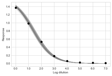
Looking at samples from the posterior distribution tells you how confident the model is in the model fit. Sparser data or data that aren’t well arranged in a sigmoid curve will yield more dispersed lines.
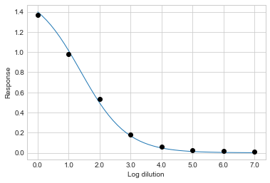
You can take the mean value of each parameter from the posterior distribution and plot the resulting sigmoid curve by passing mean=True:
sigmoid.plot_sample("21-P0004-v001sr01", mean=True)
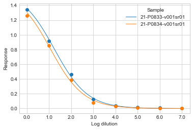
To visualize multiple samples at once, pass a list of sample names to plot_samples():
sigmoid.plot_samples(["21-P0833-v001sr01", "21-P0834-v001sr01"])
Or, to show all samples use plot_all_samples():
sigmoid.plot_all_samples()
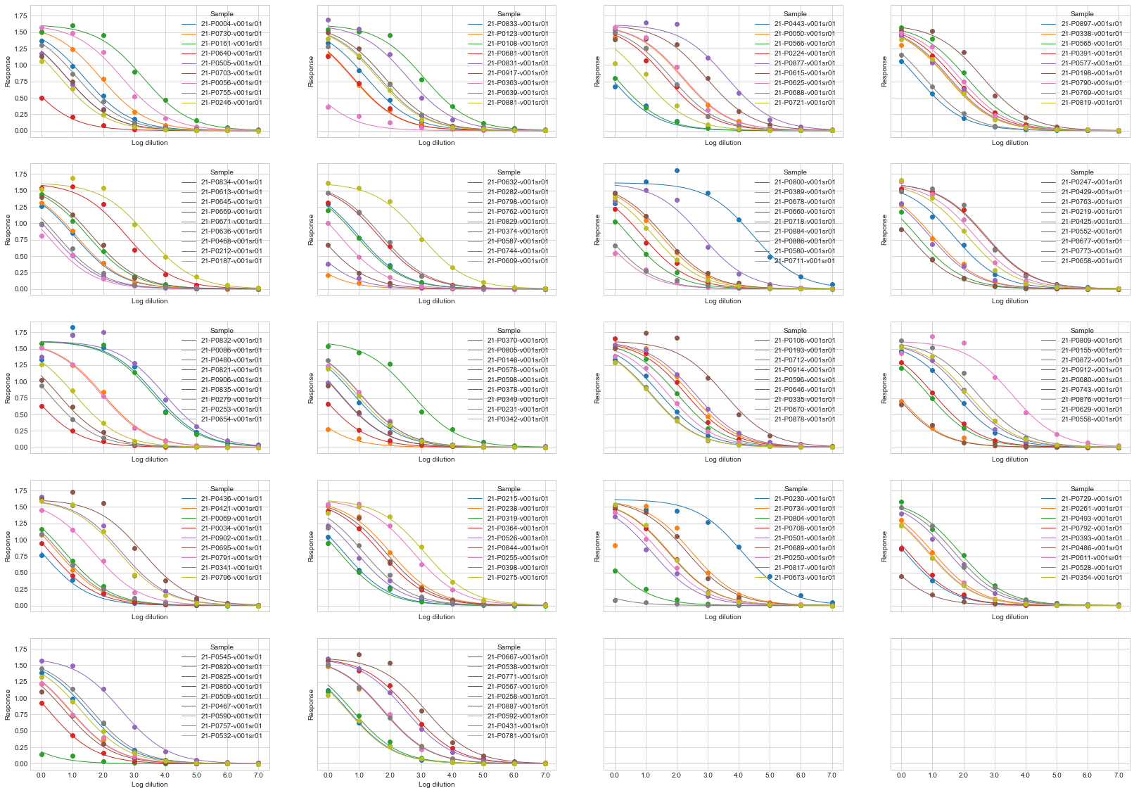
See the matplotlib documentation for help on customizing and saving figures.
Inflection titers
The degree to which a sigmoid curve is shifted left or right on the x-axis is often the point of interest to compare between samples.
This is described by the inflection point of the curve, calculated by inflections():
df_inflections = sigmoid.inflections(hdi_prob=0.95)
df_inflections.head().round(2)
sample |
mean |
median |
hdi low |
hdi high |
|---|---|---|---|---|
21-P0425-v001sr01 |
0.91 |
0.91 |
0.78 |
1.04 |
21-P0917-v001sr01 |
1.82 |
1.82 |
1.7 |
1.96 |
21-P0796-v001sr01 |
2.51 |
2.51 |
2.39 |
2.64 |
21-P0680-v001sr01 |
2.04 |
2.04 |
1.91 |
2.17 |
21-P0800-v001sr01 |
4.47 |
4.47 |
4.35 |
4.6 |
hdi low and hdi high refer to the low and high boundary of the Highest Density Interval (HDI).
An HDI is the narrowest set of parameter values that contain a certain mass of the posterior probability density - it is a type of confidence interval for a parameter.
Here, we specified an HDI probability of 0.95 (which is also the default value for the inflections() method).
Note, there is nothing particularly special about a value of 0.95
Values in this DataFrame are on the log dilution scale; i.e. they tell you the position in the dilution series of the inflection point.
To get values on the dilution scale use index_to_titer():
df_inflection_titers = it.index_to_titer(df_inflections, start=40, fold=4)
df_inflection_titers.head().round(2)
sample |
mean |
median |
hdi low |
hdi high |
|---|---|---|---|---|
21-P0425-v001sr01 |
141.43 |
141.58 |
117.89 |
169.98 |
21-P0917-v001sr01 |
501.36 |
501.69 |
422.53 |
601.65 |
21-P0796-v001sr01 |
1294.1 |
1294.03 |
1102.35 |
1544.14 |
21-P0680-v001sr01 |
676.47 |
676.82 |
563.92 |
807.78 |
21-P0800-v001sr01 |
19699.43 |
19744.58 |
16530.67 |
23644.44 |
Endpoint titers
Endpoint titers can also be computed.
An endpoint titer is the dilution at which the response drops below a certain value, known as the cut-off.
Choice of cut-off is somewhat arbitrary, but is usually some low absolute value, or a low proportion of the maximal response.
Use endpoints() to compute endpoints:
df_endpoints = sigmoid.endpoints(cutoff_proportion=0.1, hdi_prob=0.95)
df_endpoints.head().round(2)
sample |
mean |
median |
hdi low |
hdi high |
|---|---|---|---|---|
21-P0425-v001sr01 |
2.94 |
2.94 |
2.80 |
3.08 |
21-P0917-v001sr01 |
3.85 |
3.85 |
3.72 |
3.99 |
21-P0796-v001sr01 |
4.54 |
4.54 |
4.41 |
4.66 |
21-P0680-v001sr01 |
4.07 |
4.07 |
3.93 |
4.20 |
21-P0800-v001sr01 |
6.50 |
6.50 |
6.37 |
6.63 |
Like inflection points, the values in this DataFrame are on the log dilution scale.
Use index_to_titer() to put them on the dilution scale.